Modern Mathematical Statistics With Applications Second Edition Answers

Preface

Purpose

Our objective is to provide a postcalculus introdu ction to the discipline of statistics

that

• Has mathematical integrity and contains some underlying theory.

• Shows students a broad range of applications involving real data.

• Is very current in its selection of topics.

• Illustrates the importance of statistical software.

• Is accessible to a wide audience, including mathematics and statistics majors

(yes, there are a few of the latter), prospective engineers and scientists, and those

business and social science majors interested in the quantitative aspects of their

disciplines.

A number of currently available mathematical statistics texts are heavily

oriented toward a rigorous mathematical development of probability and statistics,

with much emphasis o n theorems, proofs, and derivations. The focus is more on

mathematics than on statist ical practice. Even when applied material is included,

the scenarios are often contrived (many examples and exercises involving dice,

coins, cards, widgets, or a comparison of treatment A to treatment B).

So in our exposition we have tried to achieve a balance between mathemati-

cal foundations and statistica l practice. Some may feel discomfort on grounds that

because a mathematical statistics course has traditionally been a feeder into gradu-

ate programs in statistics, students coming out of such a course must be well

prepared for that path. But that view presumes that the mathematics will provide

the hook to get students interested in our discipline. This may happen for a few

mathematics majors. However, our experience is that the application of statistics to

real-world problems is far more persuasi ve in getting quantitatively oriented

students to pursue a career or take further coursework in statistics. Let's first

draw them in with intriguing problem scenarios and applications. Opportunities

for exposing them to mathematical foundations will follow in due course. We

believe it is more important for students coming out of this course to be able to

carry out and interpret the results of a two-sample t test or simple regression

analysis than to manipulate joint moment generating functions or discourse on

various modes of convergence.

Content

The book certainly does include core material in probability (Chapter 2), random

variables and their distributions (Chapters 3–5), and sampling theo ry (Chapter 6).

But our desire to balance theory with application/data analysis is reflected in the

way the book starts out, with a chapter on descriptive and exploratory statistical

techniques rather than an immediate foray into the axioms of probability and their

consequences. After the distributional infrastructure is in place, the remaining

statistical chapters cover the basics of inference. In addition to introducing core

ideas from estimation and hypothesis testing (Chapters 7–10), there is emphasis on

checking assumptions and examining the data prior to formal analysis. Modern

topics such as bootstrapping, permutation tests, residual analysis, and logistic

regression are included. Our treatment of regression, analysis of variance, and

categorical data analysis (Chapters 11–13) is definitely more oriented to dealing

with real data than with theoretical properties of models. We also show many

examples of output from commonly used statistical software packages, something

noticeably absent in most other books pitched at this audience and level.

Mathematical Level

The challenge for students at this level should lie with mastery of statistical

concepts as well as with mathematical wizardry. Consequently, the mathematical

prerequisites and demands are reasonably modest. Mathematical sophistication and

quantitative reasoning ability are, of course, crucial to the enterpris e. Students with

a solid grounding in univa riate calculus and some exposure to multivariate calculus

should feel comfortable with what we are asking of them. The several sections

where matrix algebra appears (transformations in Chapter 5 and the matrix approach

to regression in the last section of Chapter 12) can easily be deemphasized or

skipped entirely.

Our goal is to redress the balance between mathematics and statistics by

putting more emphasis on the latter. The concepts, arguments, and notation

contained herein will certainly stretch the intellects of many students. And a solid

mastery of the material will be required in order for them to solve many of the

roughly 1,300 exercises included in the book. Proofs and derivations are include d

where appropriate, but we think it likely that obtaining a conceptual understanding

of the statistical enterprise will be the major challenge for readers .

Recommended Coverage

There should be more than enough material in our book for a year-long course.

Those wanting to emphasize some of the more theoretical aspects of the subject

(e.g., moment generating functions, conditional expectation, transformations, order

statistics, sufficiency) should plan to spend correspondingly less time on inferential

methodology in the latter part of the book. We have opted not to mark certain

sections as optional, preferring instead to rely on the experience and tastes of

individual instructors in deciding what should be presented. We would also like

to think that students could be asked to read an occasional subsection or even

section on their own and then work exercises to demonstrate understanding, so that

not everything would need to be presented in class. Remember that there is never

enough time in a course of any duration to teach students all that we'd like them to

know!

Acknowledgments

We gratefully acknowledge the plentiful feedback provided by reviewers and

colleagues. A special salute goes to Bruce Trumbo for going way beyond his

mandate in providing us an incredibly thoughtful review of 40+ pages containing

Preface xi

many wonderful ideas and pertinent criticisms. Our emphasis on real data would

not have come to fruition without help from the many individuals who provided us

with data in published sources or in personal communications. We very much

appreciate the editorial and production services provided by the folks at Springer, in

particular Marc Strauss, Kathryn Schell, and Felix Portnoy.

A Final Thought

It is our hope that students completing a course taught from this book will feel as

passionately about the subject of statistics as we still do after so many years in the

profession. Only teachers can really appreciate how gratifying it is to hear from a

student after he or she has completed a course that the experience had a positive

impact and maybe even affected a career choice.

Jay L. Devore

Kenneth N. Berk

xii Preface

CHAPTER ONE

Overview

and Descriptive

Statistics

Introduction

Statistical concepts and methods are not only useful but indeed often indis-

pensable in understanding the world around us. They provide ways of gaining

new insights into the behavior of many phenomena that you will encounter in your

chosen ﬁeld of specialization.

The discipline of statistics teaches us how to make intelligent judgments

and informed decisions in the presence of uncertainty and variation. Without

uncertainty or variation, there would be little need for statistical methods or statis-

ticians. If the yield of a crop were the same in every ﬁeld, if all individuals reacted

the same way to a drug, if everyone gave the same response to an opinion survey,

and so on, then a single observation would reveal all desired information.

An interesting example of variation arises in the course of performing

emissions testing on motor vehicles. The expense and time requirements of the

Federal Test Procedure (FTP) preclude its widespread use in vehicle inspection

programs. As a result, many agencies have developed less costly and quicker tests,

which it is hoped replicate FTP results. According to the journal article "Motor

Vehicle Emissi ons Variability" (J. Air Waste Manage. Assoc., 1996: 667–675), the

acceptance of the FTP as a gold standard has led to the widespread belief that

repeated measurements on the same vehicle would yield identical (or nearly

identical) results. The authors of the article applied the FTP to seven vehicles

characterized as "high emitters." Here are the results of four hydrocarbon and

carbon dioxide tests on one such vehicle:

HC (g/mile) 13.8 18.3 32.2 32.5

CO (g/mile) 118 149 232 236

J.L. Devore and K.N. Berk, Modern Mathematical Statistics with Applications, Springer Texts in Statistics,

DOI 10.1007/978-1-4614-0391-3_1,

Springer Science+Business Media, LLC 2012

The substantial variation in both the HC and CO measurements casts considerable

doubt on conventional wisdom and makes it much more difﬁcult to make precise

assessments about emissions levels.

How can statistical tech niques be used to gather information and draw

conclusions? Suppose, for example, that a biochemist has developed a medication

for reli eving headaches. If this medication is given to different individuals, varia-

tion in conditions and in the people themselves will result in more substantial

relief for some individuals than for others. Methods of statistical analysis could

be used on data from such an experiment to determine on the average how much

relief to expect.

Alternatively, suppose the biochemist has developed a headache medication

in the belief that it will be superior to the currently best medication. A comparative

experiment could be carried out to investigate this issue by giving the current

medication to some headache sufferers and the new medication to others. This

must be done with care lest the wrong conclusion emerge. For example, perh aps

really the two medications are equally effective. However, the new medication may

be applied to people who have less severe headaches and have less stressful lives.

The investigator would then likely observe a difference between the two medica-

tions attributable not to the medications themselves, but to a poor choice of test

groups. Statistics offers not only methods for analyzing the results of experiments

once they have been carried out but also suggestions for how experiments can

be performed in an efﬁcient manner to lessen the effects of variation and have a

better chance of producing correct conclusions.

1.1

Populations and Samples

We are constantly exposed to collections of facts, o r data, both in our professional

capacities and in everyday activities. The discipline of statistics provides methods

for organizing and summarizing data and for drawing conclusions based on infor-

mation contain ed in the data.

An investigation will typically focus on a well-defined collection of

objects constituting a population of interest. In one study, the population might

consist of all gelatin capsules of a particular type produced during a specified

period. Another investigation might involve the population consisting of all indi-

viduals who received a B.S. in mathematics during the most recent academic year.

When desired information is available for all objects in the population, we have

what is called a census . Constraints on time, money, and other scarce resources

usually make a census impractical or infeasible. Instead, a subset of the popula-

tion—a sample—is selected in some prescribed manner. Thus we might obtain

a sample of pills from a particular production run as a basis for investigating

whether pills are conforming to manufacturing specifications, or we might select

a sample of last year's graduates to obtain feedback about the quality of the

curriculum.

2 CHAPTER 1 Overview and Descriptive Statistics

We are usually interested only in certain characteristics of the objects in a

population: the amount of vitamin C in the pill, the gender of a mathematics

graduate, the age at which the individual g raduated, and so on. A characteristic

may be categorical, such as gender or year in college, or it may be numerical in

nature. In the former case, the value of the characteristic is a category (e.g., female

or sophomore), whereas in the latter case, the value is a number (e.g., age ¼ 23

years or vitamin C content ¼ 65 mg). A variable is any characteristic whose

value may change from one object to another in the population. We shall initially

denote variables by lowercase letters from the end of our alphabet. Examples

include

x ¼ brand of calculator owned by a student

y ¼ number of major defects on a newly manufactured automobile

z ¼ braking distance of an automobile under specified conditions

Data comes from making observations either on a single variable or simultaneously

on two or more variables. A univariate data set consists of observations on a

single variable. For example, we might consider the type of computer, laptop (L)

or desktop (D), for ten recent purchases, resulting in the categorical data set

DLLLDLLDLL

The following sample of lifetimes (hours) of brand D batteries in flashlights is a

numerical univariate data set:

5: 65 :16 :26 :05 :86 :55 :85 : 5

We have bivariate data when observat ions are made on each of two variables.

Our data set might consist of a (height, weight) pair for each basketball player on

a team, with the first observation as (72, 168), the second as (75, 212), and so on.

If a kinesiologist determines the values of x ¼ recuperation time from an injury and

y ¼ type of injury, the resulting data set is bivariate with one variable numerical

and the other categorical. Multivariate data arises when observations are made

on more than two variables. For example, a research physician might determine

the systolic blood pressure, diastolic blood pressure, and serum cholesterol level

for each patient participating in a study. Each observation would be a triple of

numbers, such as (120, 80, 146). In many multivariate data sets, some variables

are numerical and others are categorical. Thus the annual automobile issue of

Consumer Reports gives values of such variables as type of vehicle (small, sporty,

compact, midsize, large), city fuel efficiency (mpg), highway fuel efficiency

(mpg), drive train type (rear wheel, front wheel, four wheel), and so on.

Branches of Statistics

An investigator who has collected data may wish simply to summarize and

describe important features of the data. This entails using methods from descriptive

statistics. Some of these methods are graphical in nature; the construction of

histograms, boxplots, and scatter plots are primary examples. Other descriptive

methods involve calculation of numerical summary measures, such as means,

1.1 Populations and Samples 3

standard deviations, and correlation coefficients. The wide availability of

statistical computer software packages has made these tasks much easier to

carry out than they used to be. Computers are much more efficient than

human beings at calculation and the creation of pictures (once they have

received appropriate instructions from the user!). This means that the investiga-

tor doesn't have to expend much effort on "grunt work" and will have more

time to study the data and extract important messages. Throughout this book,

we will present output from various packages such as MINITAB, SAS, and R.

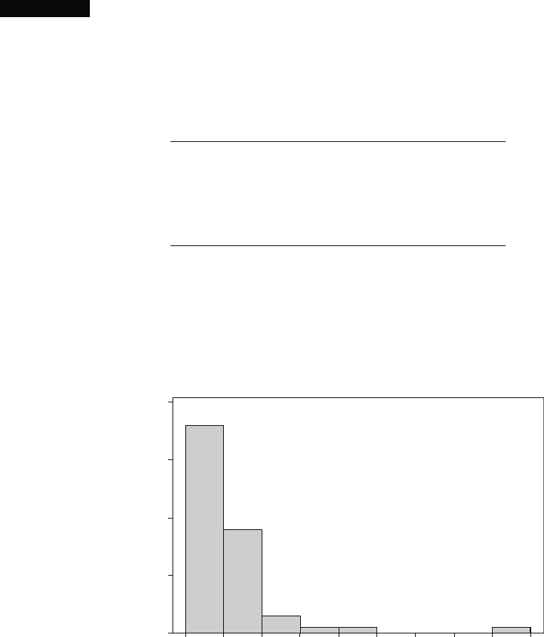
Example 1.1 Charity is a big business in the United States. The website charitynavigator.

com gives information on roughly 5500 charitable organizations, and there are

many smaller charities that fly below the navigator's radar screen. Some charities

operate very efficiently, with fundraising and administrative expenses that are

only a small percentage of total expenses, whereas others spend a high percentage

of what they take in on such activities. Here is data on fundrai sing expenses as

a percentage of total expenditures for a random sample of 60 charities:

6.1 12.6 34.7 1.6 18.8 2.2 3.0 2.2 5.6 3.8

2.2 3.1 1.3 1.1 14.1 4.0 21.0 6.1 1.3 20.4

7.5 3.9 10.1 8.1 19.5 5.2 12.0 15.8 10.4 5.2

6.4 10.8 83.1 3.6 6.2 6.3 16.3 12.7 1.3 0.8

8.8 5.1 3.7 26.3 6.0 48.0 8.2 11.7 7.2 3.9

15.3 16.6 8.8 12.0 4.7 14.7 6.4 17.0 2.5 16.2

Without any organization, it is difficult to get a sense of the data's most promi-

nent features: what a typical (i.e., representative) value might be, whether values

are highly concentrated about a typical value or quite dispersed, whether there

are any gaps in the data, what fraction of the values are less than 20%, and so on.

Figure 1.1 shows a histogram. In Section 1.2 we will discuss construction and

interpretation of this graph. For the moment, we hope you see how it describes the

10 20 30 40 50 60 70 80 900

Frequency

FundRsng

Figure 1.1 A MINITAB histogram for the charity fundraising % data

CHAPTER 1 Overview and Descriptive Statistics

way the percentages are distributed over the range of possible values from 0 to 100.

Of the 60 charities, 36 use less than 10% on fundraising, and 18 use between 10%

and 20%. Thus 54 out of the 60 charities in the sample, or 90%, spend less than 20%

of money collected on fundraising. How much is too much? There is a delicate

balance; most charities must spend money to raise money, but then money spent on

fundraising is not available to help beneficiaries of the charity. Perhaps each

individual giver should draw his or her own line in the sand.

■

Having obtained a sample from a population, an investigator would fre-

quently like to use sample information to draw some type of conclu sion (make an

inference of some sort) about the population. That is, the sample is a means to an

end rather than an end in itself. Techniques for generalizing from a sample to a

population are gathered within the branch of our discipline called inferential

statistics.

Example 1.2 Human measurements provide a rich area of application for statistical methods.

The article "A Longitudinal Study of the Development of Elementary School Chil-

dren's Private Speech" (Merrill-Palmer Q., 1990: 443–463) reported on a study of

children talking to themselves (private speech). It was thought that private speech

would be related to IQ, because IQ is supposed to measure mental maturity, and it

was known that private speech decreases as students progress through the primary

grades. The study included 33 students whose first-grade IQ scores are given here:

082 096 099 102 103 103 106 107 108 108 108 108 109 110 110 111 113

113 113 113 115 115 118 118 119 121 122 122 127 132 136 140 146

Suppose we want an estimate of the average value of IQ for the first graders

served by this school (if we conceptualize a population of all such IQs, we are

trying to estimate the population mean). It can be shown that, with a high degree

of confidence, the population mean IQ is between 109.2 and 118.2; we call this

a confide nce interval or interval estimate. The interval suggests that this is an above

average class, because the nationwide IQ average is around 100.

■

The main focus of this book is on presenting and illustrating methods of

inferential statistics that are useful in research. The most important types of inferen-

tial procedures—point estimation, hypothesis testing, and estimation by confidence

intervals—are introduced in Chapters 7–9 and then used in more complicated settings

in Chapters 10–14. The remainder of this chapter presents methods from descriptive

statistics that are most used in the development of inference.

Chapters 2–6 present material from the discipline of probability. This material

ultimately forms a bridge between the descriptive and inferential techniques.

Mastery of probability leads to a better understanding of how inferential procedures

are developed and used, how statistical conclusions can be translated into everyday

language and interpreted, and when and where pitfalls can occur in applying the

methods. Probability and statistics both deal with questions involving populations

and samples, but do so in an "inverse manner" to each other.

In a probability problem, properties of the population under study are

assumed known (e.g., in a numerical population, some specified distribution of

the population values may be assumed), and questions regarding a sample taken

1.1 Populations and Samples 5

from the population are posed and answered. In a statistics problem, characteristics

of a sample are available to the experimenter, and this information enables the

experimenter to draw conclusions about the population. The relationship between

the two disciplines can be summarized by saying that probability reasons from

the population to the sample (deductive reasoning), whereas inferential statistics

reasons from the sample to the population (inductive reasoning). This is illustrated

in Figure 1.2.

Before we can understand what a particular sample can tell us about the

population, we should first understand the uncerta inty associated with taking a

sample from a given population. This is why we study probability before statistics.

As an example of the contrasting focus of probability and inferential statis-

tics, consider drivers' use of manual lap belts in cars equipped with automatic

shoulder belt systems. (The artic le "Automobile Seat Belts: Usage Patterns in

Automatic Belt Systems," Hum. Factors, 1998: 126–135, summarizes usage

data.) In probability, we might assume that 50% of all drivers of cars equipped in

this way in a certain metropolitan area regularly use their lap belt (an assumption

about the population), so we might ask, "How likely is it that a sample of 100 such

drivers will include at least 70 who regularly use their lap belt?" or "How many

of the drivers in a sample of size 100 can we expect to regularly use their lap belt?"

On the other hand, in inferential statistics we have sample information available; for

example, a sample of 100 drivers of such cars revealed that 65 regularly use their lap

belt. We might then ask, "Does this provide substantial evidence for concluding that

more than 50% of all such drivers in this area regularly use their lap belt?" In this

latter scenario, we are attempting to use sample information to answer a question

about the structure of the entire population from which the sample was selected.

Suppose, though, that a study involving a sample of 25 patients is carried out

to investigate the efficacy of a new minimally invasive method for rotator cuff

surgery. The amount of time that each individual subsequently spends in physical

therapy is then determined. The resulting sample of 25 PT times is from a popula-

tion that does not actually exist. Instead it is convenient to think of the population as

consisting of all possible time s that might be observed under similar experimental

conditions. Such a population is referred to as a conceptual or hypothetical popula-

tion. There are a number of problem situations in which we fit questions into the

framework of inferential statistics by conceptualizing a population.

Sometimes an investigator must be very cautious about generalizing from

the circumstances under which data has been gathered. For example, a sample of

five engines with a new design may be experimentally manufactured and tested to

investigate efficiency. These five could be viewed as a sample from the conceptual

population of all prototypes that could be manufactured under similar conditions,

but not necessarily as representative of the population of units manufactured once

regular production gets under way. Methods for usin g sample information to draw

Population

Probability

Inferential

statistics

Sample

Figure 1.2 The relationship between probability and inferential statistics

CHAPTER 1 Overview and Descriptive Statistics

conclusions about future production units may be problematic. Similarly, a new

drug may be tried on patients who arrive at a clinic, but there may be some question

about how typical these patients are. They may not be representative of patients

elsewhere or patients at the clinic next year. A good exposition of these issues is

contained in the article "Assumptions for Statistical Inference" by Gerald Hahn and

William Meeker (Amer. Statist., 1993: 1–11).

Collecting Data

Statistics deals not only with the organization and analysis of data once it has been

collected but also with the development of techniques for collecting the data. If data

is not properly collected, an investigator may not be able to answer the questions

under consideration with a reasonable degree of confidence. One common problem

is that the target population—the one about which conclusions are to be drawn—

may be different from the population actually sampled. For example, advertisers

would like various kinds of information about the television-viewing habits of

potential customers. The most systematic information of this sort comes from

placing monit oring devices in a small number of homes across the United States.

It has been conjectured that placement of such devices in and of itself alters viewing

behavior, so that characteristics of the sample may be different from those of the

target population.

When data collection entails selecting individuals or objects from a list, the

simplest method for ensuring a representative selection is to take a simple random

sample. This is one for which any particular subset of the specified size (e.g., a

sample of size 100) has the same chance of being selected. Fo r exampl e, if the list

consists of 1,000,000 serial numbers, the numbers 1, 2, ... , up to 1,000,000 could

be placed on identical slips of paper. After placing these slips in a box and

thoroughly mixing, slips could be drawn one by one until the requisite sample

size has been obtained. Alternatively (and much to be preferred), a table of random

numbers or a computer's random number generator could be employed.

Sometimes alternative sampling methods can be used to make the selection

process easier, to obtain extra information, or to increase the degree of confidence

in conclusions. One such method, stratified sampling, entails separating the

population units into nonoverlapping groups and taking a sample from each one.

For example, a manufacturer of DVD players might want information about

customer satisfaction for units produced during the previous year. If three different

models were manufactured and sold, a separate sample could be selected from each

of the three corresponding strata. This would result in information on all three

models and ensure that no one model was over- or underrepresented in the entire

sample.

Frequently a "convenience" sample is obtaine d by selecting individuals or

objects without systematic randomization. As an example, a collection of bricks

may be stacked in such a way that it is extremely difficult for those in the center to

be selected. If the bricks on the top and sides of the stack were somehow different

from the others, resu lting sample data would not be representative of the popula-

tion. Often an investigator will assume that such a convenience sample approx-

imates a random sample, in which case a statistician's repertoire of inferential

methods can be used; however, this is a judgment call. Most of the methods

discussed herein are based on a variation of simple random sampling described in

Chapter 6.

1.1 Populations and Samples 7